Two-Phase Flow
Explore two-phase flow correlations and apply them to real networks.
Pipeline Engineer offers two algorithms that allow users to play around with two-phase flow algorithms.
Two-Phase Network Elements
Users can create a two-phase source or sink layer from the Network Component Creator.
Liquid Mass Flow Rate (l_mdot_kg_per_s) and a Gas Mass Flow Rate (g_m_dot_kg_per_s) quantities can be set on these layers.
In order to run either of the two algorithms mentioned in this example, the network being analysed must have at least one two-phase source layer or one two-phase sink layer.
Two-Phase Correlations
The literature regarding two-phase flow is quite extensive. Out of the box, Pipeline Engineer offers three two-phase correlations - these being the Homogeneous Model, Lockhart-Martinelli Model and the Beggs & Brill Model.
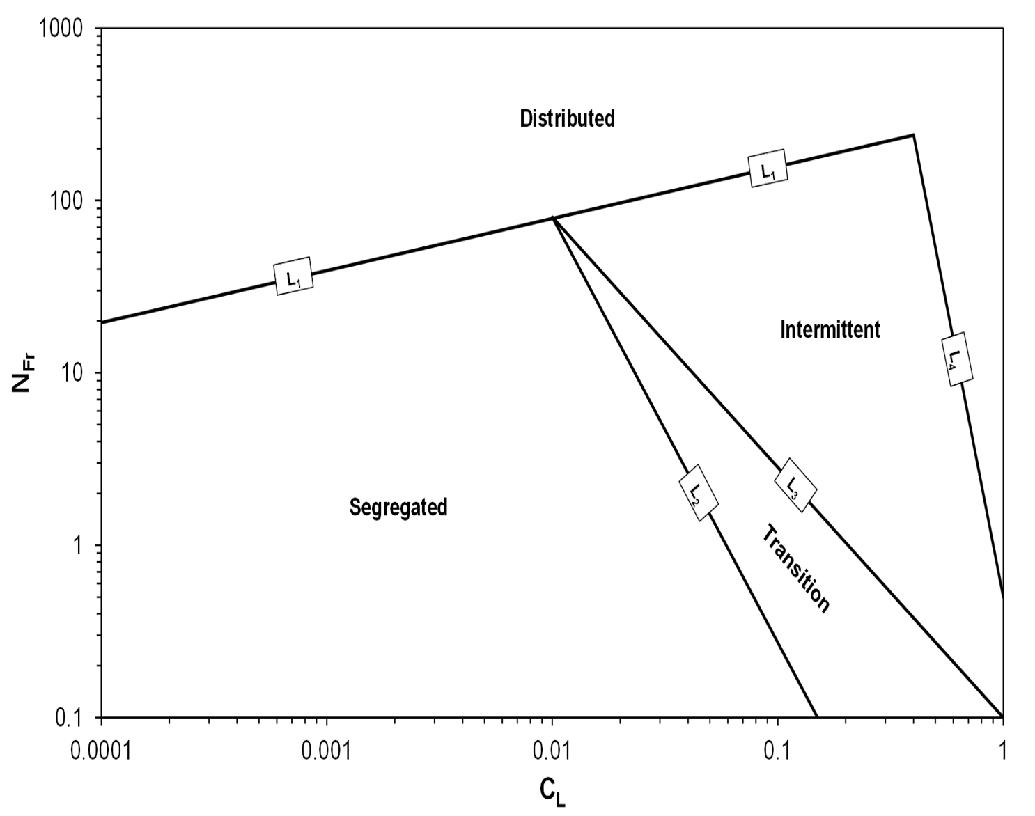
Algorithms
Two-Phase Flow (Node-to-Node)
The Two-Phase Flow (Node-to-Node) algorithm works similarly to the Pipeflow function. The correlation will be applied between the nodes defined in the network.
The main benefit of this algorithm is that quick comparisons with existing literature can be done to determine whether a correlation has been implemented correctly.
Fluidflow Comparison
As an example, Pipeline Engineer was used to recreate a case demonstrated on the FluidFlow by Flite Results Verification Page.
The problem stated in the above example is as follows:-
Calculate the pressure loss in a two-phase system pipeline (50.8mm diameter) which features an air input of 240.7 m3/h at 26.6 °C and water at 5.677 m3/h at 26.6 °C.
Firstly, these quantities were converted in the appropriate units for Pipeline Engineer:-
- 5.677 * (996 / 3600) = 1.57 kg/s of water
- 240.7 * (1.18/3600) = 0.08 kg/s of air
The length of the pipe was selected as 1m or 0.001km, the diameter was 0.0508m and the roughness was set at 0.063mm.
The homogenous model was selected for this example.

Tabulated below is a comparison of the selectedd example against the data from the published source, FluidFlow and Pipeline Engineer.
| Description | Published Data | FluidFlow Results | Pipeline Engineer Results |
|---|---|---|---|
| Pressure loss (kPa/m) | 5.15 | 5.78 | 5.85 |
As is evident, the value calculated by Pipeline Engineer compares well with the answer calculated by FluidFlow.
Two-Phase Flow
The Two-Phase Flow Algorithm is intended to be more robust and representative of real systems.
As with the Incompressible Flow Algorithm, pressure drop is calculated for each user defined length of pipe. This has the added benefit of allowing the density of the gas to be re-calculated, as this in turn will change the gas volume fraction.
Pictured below is an example - the plot on the bottom represents the elevation profile of the pipeline in question.
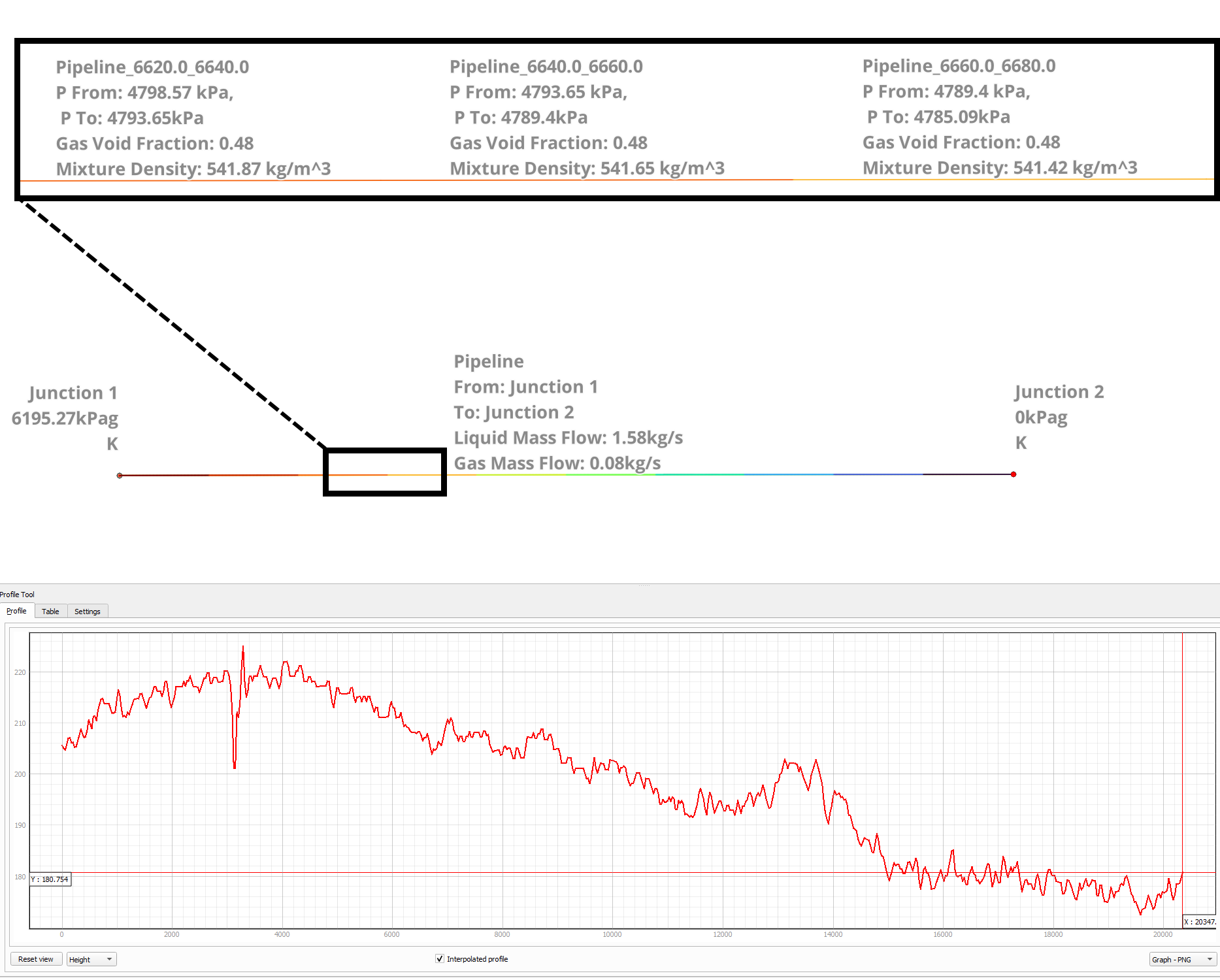
As is evident, the section-by-section pressure layer contains a newly calcuated gas void fraction for the new gas density that is updated iteratively.